Let's try regression on the auto dataset:
regfit.full <- regsubsets(price~., auto)
It doesn't work because by default, exhaustive search is performed.
This requires lots of permutations, so you have to set really.big=TRUE if you want this.
But let's just make things simpler by carving out a subset of variables:
autosmall <- auto[,c(2,3,5,6,7,8,9,10,11)]
regfit.full <- regsubsets(price ~ . , autosmall) # the . indicates we want all variables to be considered.
summary(regfit.full)
regfit.fwd <- regsubsets(price~., autosmall, method="forward") # forward stepwise selection
regfit.bwd <- regsubsets(price~., autosmall, method="backward") # backward stepwise selection
coef(regfit.fwd,3) # gives the coefficients for regfit.fwd for the optimal 3-variable model
Recall that we actually need to split our dataset into a training set and test set. This is how we can do it:
set.seed(1)
train <- sample(c(TRUE, FALSE),nrow(autosmall),rep=TRUE)
# if we wanted 75% of observations to be in training set, we can do the below:
# train <- sample(c(TRUE, FALSE),nrow(autosmall),rep=TRUE, prob = c(0.75, 0.25))
test <- (!train)
# another way of allocating the training/test sets:
# train <- sample(1:nrow(autosmall), nrow(autosmall)/2)
# test <- (-train)
# autosmall.test <- autosmall[test]
# (notice that test contains all negative numbers, so all "train" observations are excluded)
To keep things simple, we didn't do cross validation (as well as regularization).
Here's how to do cross-validation:
regfit.full <- regsubsets(price~., autosmall[train,])
reg.summary <- summary(regfit.full) # for convenience
names(reg.summary)
For model selection, it'll be useful to plot how RSS (and other measures such as adjusted R-sq) varies with number of variables:
par(mfrow = c(1,2)) # sets a 1 row by 2 column plot
plot(reg.summary$rss,xlab="# of Var", ylab="RSS", type="l")
(m1 <- which.min(reg.summary$rss))
points(m1,reg.summary$rss[m1], col="red",cex=2,pch=20)
# cex refers to the dot thickness
plot(reg.summary$adjr2,xlab="# of Var", ylab="Adj R2", type="l")
(m1 <- which.max(reg.summary$adjr2))
points(m2,reg.summary$adjr2[m2], col="red",cex=2,pch=20)
plot(regfit.full, scale="r2")
Now we need to see MSE on the test set. First off, use model.matrix to generate the "X" matrix for the test set:
test.mat <- model.matrix(price~., data=autosmall[test,])
val.errors = rep(NA,8) # generates the empty MSE matrix
for (i in 1:8) {
coefi <- coef(regfit.full, id=i) # takes the coefficients from the optimal model with i variables
pred <- test.mat[,names(coefi)] %*% coefi # generate predicted values of each observation
val.errors[i] <- mean((autosmall$price[test] - pred)^2) # generate MSE for i-th model
}
val.errors
#[1] 7781131 9856769 10060398 9574022 9421108 9470527 9269711 8942316
(v <- which.min(val.errors))
#[1] 1
# so we choose model with 1 variable (weight only)
coef(regfit.full, v)
#(Intercept) weight
#-426.910662 2.251572
We can also write a function, which will come in useful for k-fold cross validation
predict.regsubsets <- function(object, newdata, id, ...) {
form <- as.formula(object$call[[2]]) # takes the second item from object$call list
# call is part of regfit.full
# the second item within the list is the relevant variables
mat <- model.matrix(form, newdata) # generates the required X matrix using the formula
coefi <- coef(object, id=id) # the X variable COEFFICIENTS of the optimal model
xvars <- names(coefi) # these are the X variables of the optimal model
mat[,xvars] %*% coefi # generates predicted values (by looking at the relevant columns only)
}
# 10-fold cross validation
k = 10
set.seed(1)
folds = sample(1:k, nrow(autosmall), replace=TRUE)
# if an observation is labelled 'i', it will be part of the i-th fold.
# e.g. an observation that is labelled 3 will be left out of the 3rd round of cross validation
cv.errors = matrix(NA,k,8, dimnames=list(NULL, paste(1:8)))
# sets up a k by 8 matrix filled with NA's.
# columns are named 1 to 8
# armed with our new predict() method, we can:
for (j in 1:k) {
# obtain the required coefficients
best.fit <- regsubsets(price ~ . , data=autosmall[folds != j,])
# note: if you have more than 8 variables you will need to specify nvmax in the above command
for (i in 1:8) {
# now, calculate MSE using the i-th fold
pred <- predict(best.fit, autosmall[folds == j,],id=i)
# since best.fit is of class regsubsets, the predict command that was created will work on it.
cv.errors[j,i] <- mean((autosmall$price[folds == j] - pred)^2)
}
}
(mean.cv.errors <- apply(cv.errors,2,mean))
Let's plot MSE of the CV dataset.
par(mfrow=c(1,1))
plot(mean.cv.errors, type='b')
Sunday, July 12, 2015
Overview of Machine Learning Techniques in R
Whenever we do something as simple as a Google search, we benefit from machine learning. Demand is high for those with machine learning skills - a search of LinkedIn reveals 9,369 results for "machine learning".
This post gives an overview of packages (and functions within those packages) one can use to conduct machine learning techniques. A lot of this material is drawn from the fourth edition of the textbook Introduction to Statistical Learning.
This post gives an overview of packages (and functions within those packages) one can use to conduct machine learning techniques. A lot of this material is drawn from the fourth edition of the textbook Introduction to Statistical Learning.
- Linear regression
Library: leaps
Functions: regsubsets
- Decision trees
- Support Vector Machines
- Unsupervised learning
Subsequent posts will elaborate on these in more detail.
Apply, lapply, sapply, tapply in R
How can we use R to efficiently calculate key statistics such as the mean?
Let's play with the auto dataset to see how.
apply(cbind(auto$price,auto$length,auto$weight),2,mean) # finds simple means
apply(auto,2,mean) would not work because some arguments are non-numeric.
Instead, one can try apply(auto[,c(2,3)],2,mean).
If you wanted to find out the number of values each variable took, this would be simple:
apply(auto, 2, function (x) length(unique(x)))
The second argument (2) tells R to work column-by-column. Had 1 been specified, R would have worked row-by-row. You can also use the sapply function, which by default returns a vector:
sapply(auto, function(x) length(unique(x)))
If we wanted the output in terms of a list, we could use lapply:
lapply(auto, function(x) length(unique(x)))
What if we wanted disaggregated statistics? For example, we might want to know what is the mean price of foreign cars, as well as the mean price of domestic cars. We can use
tapply(auto$price, auto$foreign, mean)
Which would be similar to Excel's PivotTable. The by function is also acceptable:
by(auto$price, auto$foreign, mean)
What if the variable has NA values? For example, by(auto$price, auto$foreign, mean) returns us the unglamorous
auto$foreign: Domestic
[1] NA
-----------------
auto$foreign: Foreign
[1] NA
This was because the rep78 contained missing values. We can easily handle this:
tapply(auto$rep78, auto$foreign, function(x) mean(x, na.rm=TRUE))
or
by(auto$rep78, auto$foreign, function(x) mean(x, na.rm=TRUE))
And what if we wanted to restrict attention to cars with prices above $1000:
tapply(auto$rep78, auto$foreign, function(x) mean(x[auto$price > 10000],na.rm=TRUE))
or
by(auto$rep78, auto$foreign, function(x) mean(x, na.rm=TRUE))
Yet another way is to subset the data first:
m <- subset(auto, !is.na(auto$rep78) & auto$price > 10000)
by(m$rep78, m$foreign, mean)
Useful resources for learning R
- R-bloggers is a collection of R blogs.
- UCLA has a comprehensive guide
- Try tryr
Monday, July 6, 2015
Extracting JSON data in R
Increasingly, data on the internet is presented in JSON format. For the uninitiated, here's what a JSON file looks like:
{
people:[
{name:"John Smith", timings:[1,2,3]},
{name:"Adam Yu", timings:[3,2,1]},
{name:"Frank Pin", timings:[7,4,3]}
}
It's more or less a data file. The curly braces indicated named arrays (e.g. we know that we have the name and timings of each person), while the square brackets indicate ordered unnamed arrays (e.g. Frank's first timing is 7, his second timing is 4, and his third timing is 3.)
How can R analyze the data appropriately? Let's take a look at a real life example: the salaries of public servants at the City of Chicago. R has three major packages which can analyze JSON data.
These are RJSONIO, rjson, and jsonlite. The differences are minor, especially for simple JSON files.
Here, we will use the RJSONIO package.
First, let's download and install the required packages and load the required data.
install.packages("RJSONIO")library(RJSONIO)RawData <- fromJSON("https://data.cityofchicago.org/api/views/xzkq-xp2w/rows.json?accessType=DOWNLOAD")Should you have difficulty downloading the city of Chicago data, here's a link. (Note: information in the link is correct as of July 2015)You should actually display the JSON file a web browser for easier viewing. Once you've done this, you'll notice that what you're looking for is in the data section. HenceData <- RawData$datagives you most of what you need. I say most, because things like variable names aren't there. Here's an example of how you would extract a given variable:employeeNames <- sapply(Data, function(x) x[[9]])Just to check that things are working properly, we can runhead(employeeNames)In order to extract all variables efficiently, we need to define two functions.install.packages('gdata')library(gdata) # necessary for trimgrabinfo <- function(var) {print(paste("Variable", var, sep=" ")) # for aesthetics: tells you which variables have been processedsapply(Data, function(x) returnData(x,var)) # the dataset "Data" is hardcoded here and is input as parameter "x"}returnData <- function(x, var) {if (!is.null( x[[var]] )) {return ( trim( x[[var]] ))} else {return(NA)}}df <- data.frame(sapply(1:length(Data[[1]]),grabinfo), stringsAsFactors=FALSE)# Performs grabinfo for each variable in Data# you run grabinfo(1), grabinfo(2), ... grabinfo(12).## grabinfo(1) then uses sapply (again) to get values of Variable1 for all observations# likewise with grabinfo(2), and so on## in doing so, the entire dataset is transformed into a dataframeFinally, some technicalities:head(df) # Just checking that things are working againnames(df) <- sapply(1:12,function(x) RawData[['meta']][['view']][['columns']][[x]][['name']])df$`Employee Annual Salary` <- as.numeric(df$`Employee Annual Salary`) # change the variable to numericOf course, this is a very simple case. What if our JSON contains nested objects (objects within objects)? You may wish to consult this excellent guide (this blogpost took many good points from there). What if you're actually downloading a Javascript file containing JSON? Check this out.
Sunday, July 5, 2015
Linear Regression in R
Let's load the auto dataset and learn regression techniques in more detail. (For those who have not read previous posts, this is a dataset containing information about 74 cars.)
Suppose we want to find the relationship between the price and weight of a car. One way to do this is
priceweight <- lm(auto$price ~ auto$weight)
Alternatively,
priceweight <- lm(price ~ weight, data=auto)
will work as well.
The command summary(priceweight) will then display details of the regression such as coefficient estimates and p-values.
We can then visualize the data by
plot(auto$weight,auto$price)
abline(priceweight)
Notice that for plot, the first named variable takes the x axis, while the other variable takes the y axis.
The function abline draws a straight line through the plot, using the coefficients produced by the regression. You can always produce other lines if you want. For example,
abline(a=0,b=1,col='blue')
produce a straight line with an intercept of 0 and a slope of 1. In other words, this would be the model if price and weight had a 1:1 relationship (clearly not supported by the data). Notice that specifying a blue color helps to differentiate this line from the best-fit line.
If we wanted to, we could emphasize the best fit line more:
abline(priceweight, lwd = 5)
here lwd stands for linewidth. The line will be 5 units thick (the default is 1 unit thick, so we have increased the width drastically).
Squared terms
It might be reasonable to think that price is a non-linear function of weight. How can we see whether, for example, price is a quadratic function of weight?
An intuitive guess may be
priceweight2 <- lm(price ~ weight + weight^2, data=auto)
But it doesn't quite produce the results we want:
Call:
lm(formula = price ~ weight + weight^2, data = auto)
Coefficients:
(Intercept) weight
-6.707 2.044
What you actually wanted to do was this:
priceweight2 <- lm(price ~ weight + I(weight^2), data=auto)
The I() means "inhibit". In this case, without I(), ^ would be a formula operator. Using I() allows ^ to be interpreted as a arithmetic operator. If you are confused, think of it this way: ^ has a special meaning when it appears in a formula. Using I() suppresses this special meaning, and forces R to treat it in the normal way (exponential).
With this in mind, we can do standard F tests to determine if model fitness significantly improves with the addition of a squared term.
anova(priceweight,priceweight2)
Analysis of Variance Table
Model 1: price ~ weight
Model 2: price ~ weight + I(weight^2)
Res.Df RSS Df Sum of Sq F Pr(>F)
1 72 450831459
2 71 384779934 1 66051525 12.188 0.0008313 ***
---
Signif. codes: 0 ‘***’ 0.001 ‘**’ 0.01 ‘*’ 0.05 ‘.’ 0.1 ‘ ’ 1
Model fitness significantly improves. Since the null hypothesis is rejected, the test therefore lends support to the inclusion of a squared term. The test, however, is by no means definitive - a lot more things need to be considered. For example, you could run
plot(priceweight)
plot(priceweight2)
and end up with the following plots:
Linear case:

Quadratic case:

It looks like in the quadratic case, the residuals are much less correlated with the fitted values. This also suggests that a quadratic model is better.
With this in mind, we can do standard F tests to determine if model fitness significantly improves with the addition of a squared term.
anova(priceweight,priceweight2)
Analysis of Variance Table
Model 1: price ~ weight
Model 2: price ~ weight + I(weight^2)
Res.Df RSS Df Sum of Sq F Pr(>F)
1 72 450831459
2 71 384779934 1 66051525 12.188 0.0008313 ***
---
Signif. codes: 0 ‘***’ 0.001 ‘**’ 0.01 ‘*’ 0.05 ‘.’ 0.1 ‘ ’ 1
Model fitness significantly improves. Since the null hypothesis is rejected, the test therefore lends support to the inclusion of a squared term. The test, however, is by no means definitive - a lot more things need to be considered. For example, you could run
plot(priceweight)
plot(priceweight2)
and end up with the following plots:
Linear case:


It looks like in the quadratic case, the residuals are much less correlated with the fitted values. This also suggests that a quadratic model is better.
Interaction Variables
Suppose we hypothesized that the relationship between price and weight was different from foreign cars as compared to domestic cars.
Then we can use
priceweight <- lm(price ~ weight + weight:foreign, data=auto)
We might even think that being foreign has some effect, so let's throw the variable in:
priceweight <- lm(price ~ weight + weight:foreign + foreign, data=auto)
But hey, all these can be simplified:
priceweight <- lm(price ~ weight*foreign, data=auto)
Notice that weight*foreign is simply shorthand for weight + weight:foreign + foreign.
Logistic Regression
Logistic regression is an instance of generalized linear models (GLM). Notice that the variable foreign takes on only two values: domestic and foreign. Suppose (this is for the sake of giving an example), we thought that price was a predictor of a car being foreign. We can then run
nonlinear <- glm(foreign~price,data=auto,family=binomial)
summary(nonlinear)
The argument family=binomial ensures that a logistic regression is run (there are many kinds of GLMs, so we want to pick the right one. Naturally, one may be unsure over whether "Domestic" is 0 or 1, but one can easily verify this with
contrasts(auto$foreign)
which tells us that R treats "Domestic" as being equal to 0 and "Foreign" as being equal to 1.
predictedprob <- predict(nonlinear, type="response")
auto$predicted <- rep("Domestic", dim(auto)[1])
auto$predicted[predictedprob>=0.5] <- "Foreign"
table(auto$predicted,auto$foreign)
which gives us the confusion matrix
Domestic Foreign
Domestic 52 22
Foreign 0 0
The last row may not appear on your screen, but I added it for clarity. Notice that it is price is a very poor predictor of whether a car is domestic or foreign. Our model predicts that all cars are domestically produced, resulting in a large number of errors. We either need to find better predictors, or tweak the threshold above which we predict a car is of foreign origin.
Saturday, July 4, 2015
Scatterplots with ggplot2
While the standard R installation comes with basic scatterplot functions, one often needs more advanced functions. To this end, one very popular package is ggplot2, where gg refers to "grammar of graphics".
library(ggplot2)
library(choroplethr)
data(df_state_demographics)


and...

library(ggplot2)
library(choroplethr)
data(df_state_demographics)
names(df_state_demographics)
outputs
[1] "region" "total_population" "percent_white" "percent_black"
[5] "percent_asian" "percent_hispanic" "per_capita_income" "median_rent"
[9] "median_age"
Suppose we want to see the relationship between per capita income and median rent in each state. A simple way of doing this would be
ggplot(df_state_demographics, aes(x=per_capita_income, y=median_rent))
+ geom_point(shape=1)
The first argument tells us the dataset we want to use. We can then specify the x and y variables within aes. Think of aes as creating an "aesthetic", or something which allows you to specify which variables go where.
At a bare minimum, ggplot requires us to specify what shape we want the plots to take. These must be added on as a separate layer. Hence the command "+ geom_point(shape=1)". The output follows:

If we want a linear regression line, we can tack on another layer:
ggplot(df_state_demographics, aes(x=per_capita_income, y=median_rent))
+ geom_point(shape=1)
+ geom_smooth(method=lm)
which gives us

What if we don't want confidence intervals? Then we can try
ggplot(df_state_demographics, aes(x=per_capita_income, y=median_rent))
+ geom_point(shape=1)
+ geom_smooth(method=lm, se=FALSE)

Finally, what if we want to do LOESS? Just omit the arguments within geom_smooth.
ggplot(df_state_demographics, aes(x=per_capita_income, y=median_rent))
+ geom_point(shape=1)
+ geom_smooth()
Of course, we would want to make things fancier. For example, we might want to add a title. To make things simple, let's save our base plot as base_plot:
base_plot <- ggplot(df_state_demographics, aes(x=per_capita_income, y=median_rent))
+ geom_point(shape=1)
+ geom_smooth()
How can we:
1. Add a title?
base_plot + ggtitle("State per capita income and median rent")
2. Add labels?
base_plot + xlab("Per capita income ($)") + ylab("Median rent ($)")
Of course, this is just the tip of the iceberg. You may wish to see this excellent tutorial (part of this blogpost was drawn from there).
Plotting maps with choroplethr
According to the below graphic from the Sacramento Bee, Latinos have overtaken whites to become the most populous ethnic group.

Thereafter, we create the individual maps. Notice that each map is created by adding "layers" on top of each other. For example, choro_white consists of three layers:
1. county population data of whites (county_choropleth accesses df_county_demographics$value)
2. a graph title,
3. a geographical map (coord_map()), which is part of ggplot2.
df_county_demographics$value = df_county_demographics$percent_white
choro_white = county_choropleth(df_county_demographics, state_zoom="california", num_colors=1) +
ggtitle("California Counties\n Percent White") +
coord_map()
df_county_demographics$value = df_county_demographics$percent_hispanic
choro_hispanic = county_choropleth(df_county_demographics, state_zoom="california", num_colors=1) +
ggtitle("California Counties\n Percent Hispanic") +
coord_map()
df_county_demographics$value = df_county_demographics$percent_asian
choro_asian = county_choropleth(df_county_demographics, state_zoom="california", num_colors=1) +
ggtitle("California Counties\n Percent Asian") +
coord_map()


Let's use the choroplethr package to examine the racial distribution of California counties.
Let's start with the preliminaries: installing and loading the package, as well as loading the relevant datasets. We'd also need to load the ggplot2 library, which will come useful in plotting the maps.
install.packages("choroplethr")
library(choroplethr)
data(df_state_demographics)
data(df_county_demographics)
library(ggplot2)Thereafter, we create the individual maps. Notice that each map is created by adding "layers" on top of each other. For example, choro_white consists of three layers:
1. county population data of whites (county_choropleth accesses df_county_demographics$value)
2. a graph title,
3. a geographical map (coord_map()), which is part of ggplot2.
df_county_demographics$value = df_county_demographics$percent_white
choro_white = county_choropleth(df_county_demographics, state_zoom="california", num_colors=1) +
ggtitle("California Counties\n Percent White") +
coord_map()
df_county_demographics$value = df_county_demographics$percent_hispanic
choro_hispanic = county_choropleth(df_county_demographics, state_zoom="california", num_colors=1) +
ggtitle("California Counties\n Percent Hispanic") +
coord_map()
df_county_demographics$value = df_county_demographics$percent_asian
choro_asian = county_choropleth(df_county_demographics, state_zoom="california", num_colors=1) +
ggtitle("California Counties\n Percent Asian") +
coord_map()
Finally, we need to display the maps we've produced:
library(gridExtra)
grid.arrange(choro_white, choro_hispanic, choro_asian, nrow=3)
The output:
library(gridExtra)
grid.arrange(choro_white, choro_hispanic, choro_asian, nrow=3)

As is expected, the southern counties have more Hispanics.
Thursday, July 2, 2015
R for Stata users (Part 3)
In part 1 and part 2, we learned how to use R to load datasets, perform simple manipulations, and conduct linear regression.
Here, we will learn how to save work, draw scatterplots, handle dates and times, extract substrings, and encode variables. Make sure that you've opened RStudio and loaded the auto dataset.
Task #11: Save work
Once you've loaded and analyzed the auto dataset, you'll be wondering how to save it. For example, you may need to pass a CSV or Stata file to your colleague. Fortunately, R has lots of capabilities in these areas.
The following command will write a CSV file to RStudio's current working directory:
write.csv(auto, "edited_auto.csv")
If you don't know what the current working directory is, type
getwd()
(short for get working directory). You can then find your file in that directory.
Alternatively, type
write.csv(auto, "C:/Documents/edited_auto.csv")
if you have a folder called Documents and want to place it there.
Important: In R, use forward slashes instead of backward slashes when writing directory paths.
One remark is that if I wanted to have a tab separated file, I could use the more general "write.table":
write.table(auto, "C:/Documents/edited_auto.csv", sep="\t")
where \t denotes the tab symbol.
To write an Excel file, you need something called a "library". Think of a library as an add-on. It first needs to be installed
install.packages("xlsx")
where xlsx is the specific library we are instructing R to download. Thereafter, we need to load the package:
library(xlsx)
and we can then write our Excel file.
write.xlsx(auto, "C:/auto.xlsx")
the first parameter (auto) tells us the dataframe we want R to save, and the second parameter (C:/auto.xlsx) tells us where we want to save it. Notice again the use of a forward slash.
Of course, as a veteran Stata user, you may want to save something directly into a .dta file. You'll need a different library, called "foreign".
install.packages("foreign")
library(foreign)
write.dta(auto,"auto.dta")
and remember to locate auto.dta in the working directory.
Task #12: Draw scatterplots
Plotting graphs in R is pretty much an art. There are many specialized libraries which allow you draw beautiful graphs. However, for the beginner, it's best to use the simple plot function.
Let's say we've loaded the dataset and want to do a scatterplot of price against weight. We can type
plot(auto$price,auto$weight)
The scatterplot appears on the bottom right corner.

However, it's a bare scatterplot. Let's make it better looking. First off, we can label the x and y axes more appropriately:
plot(auto$price,auto$weight, xlab="Price",ylab="Weight")
We can also add a title:
plot(auto$price,auto$weight, xlab="Price",ylab="Weight", main="Price vs. Weight")
For those who want more advanced graphing, take a look at the ggplot2 and lattice libraries.
Task #13: Handle dates and times
This is a little difficult to teach using the auto dataset (since there are no dates), but you can find a good tutorial here.
Task #14: Obtain substrings
Take a look at the variable "make". Notice that it takes on values such as "AMC Concord", "AMC Pacer", "Buick Century", and so on. Let's say that the first word is the car manufacturer's name, and the second word refers to the model. How can we separate the two?
Libraries come to the rescue again.
install.packages("stringr")
library(stringr)
auto$manufacturer <- str_split_fixed(auto$make, " ",2)[,1]
auto$model <- str_split_fixed(auto$make, " ",2)[,2]
str_split_fixed is a function within the stringr library.
The first parameter tells us which dataframe column we want to split, and " " is the instruction to look for a space. The last parameter (2) means that we are expecting two columns. Finally, [,1] and [,2] refer to the first and second column respectively.
At this point, it's useful to check that you've got the desired results.
Task #15: Encoding variables.
Look at the variable "foreign". In Stata, there is the "encode" command, which will allow you to code the different string values of foreign into numeric variables.
Here, you can do
auto$foreign_dummy <- as.numeric(auto$foreign)
and you will see 1's and 2's.
Here, we will learn how to save work, draw scatterplots, handle dates and times, extract substrings, and encode variables. Make sure that you've opened RStudio and loaded the auto dataset.
Task #11: Save work
Once you've loaded and analyzed the auto dataset, you'll be wondering how to save it. For example, you may need to pass a CSV or Stata file to your colleague. Fortunately, R has lots of capabilities in these areas.
- CSV File
The following command will write a CSV file to RStudio's current working directory:
write.csv(auto, "edited_auto.csv")
If you don't know what the current working directory is, type
getwd()
(short for get working directory). You can then find your file in that directory.
Alternatively, type
write.csv(auto, "C:/Documents/edited_auto.csv")
if you have a folder called Documents and want to place it there.
Important: In R, use forward slashes instead of backward slashes when writing directory paths.
One remark is that if I wanted to have a tab separated file, I could use the more general "write.table":
write.table(auto, "C:/Documents/edited_auto.csv", sep="\t")
where \t denotes the tab symbol.
- Excel file
install.packages("xlsx")
where xlsx is the specific library we are instructing R to download. Thereafter, we need to load the package:
library(xlsx)
and we can then write our Excel file.
write.xlsx(auto, "C:/auto.xlsx")
the first parameter (auto) tells us the dataframe we want R to save, and the second parameter (C:/auto.xlsx) tells us where we want to save it. Notice again the use of a forward slash.
- Stata
Of course, as a veteran Stata user, you may want to save something directly into a .dta file. You'll need a different library, called "foreign".
install.packages("foreign")
library(foreign)
write.dta(auto,"auto.dta")
and remember to locate auto.dta in the working directory.
- SAS
If your collaborators use SAS, not to worry, the foreign package also has SAS capabilities.
write.foreign(auto, "auto.txt", "auto.sas", package="SAS")
The first parameter tells R the dataset to use and the second tells what data file to output. The third tells us to produce a file containing code to interpret the dataset. What kind of code? That's the job of the final parameter, which tells us it's SAS code that should be produced.
Task #12: Draw scatterplots
Plotting graphs in R is pretty much an art. There are many specialized libraries which allow you draw beautiful graphs. However, for the beginner, it's best to use the simple plot function.
Let's say we've loaded the dataset and want to do a scatterplot of price against weight. We can type
plot(auto$price,auto$weight)
The scatterplot appears on the bottom right corner.

However, it's a bare scatterplot. Let's make it better looking. First off, we can label the x and y axes more appropriately:
plot(auto$price,auto$weight, xlab="Price",ylab="Weight")
We can also add a title:
plot(auto$price,auto$weight, xlab="Price",ylab="Weight", main="Price vs. Weight")
For those who want more advanced graphing, take a look at the ggplot2 and lattice libraries.
Task #13: Handle dates and times
This is a little difficult to teach using the auto dataset (since there are no dates), but you can find a good tutorial here.
Task #14: Obtain substrings
Take a look at the variable "make". Notice that it takes on values such as "AMC Concord", "AMC Pacer", "Buick Century", and so on. Let's say that the first word is the car manufacturer's name, and the second word refers to the model. How can we separate the two?
Libraries come to the rescue again.
install.packages("stringr")
library(stringr)
auto$manufacturer <- str_split_fixed(auto$make, " ",2)[,1]
auto$model <- str_split_fixed(auto$make, " ",2)[,2]
str_split_fixed is a function within the stringr library.
The first parameter tells us which dataframe column we want to split, and " " is the instruction to look for a space. The last parameter (2) means that we are expecting two columns. Finally, [,1] and [,2] refer to the first and second column respectively.
At this point, it's useful to check that you've got the desired results.
Task #15: Encoding variables.
Look at the variable "foreign". In Stata, there is the "encode" command, which will allow you to code the different string values of foreign into numeric variables.
Here, you can do
auto$foreign_dummy <- as.numeric(auto$foreign)
and you will see 1's and 2's.
Tuesday, June 30, 2015
R for Stata users (part 2)
This is Part 2 of "How to convert from Stata to R". (If you haven't read Part 1, here's the link).
In this part, we will learn about sorting, generating/dropping new variables, linear regression, and post estimation commands.
If you haven't loaded the auto dataset, load it.
Task #6: Sort
While Stata has "sort", R has "order".
After you've loaded the dataset, enter
auto[order(auto$price),]
(don't forget the comma at the end!)
Notice that the dataset is sorted in ascending order:
make price mpg rep78 ...
34 Merc. Zephyr 3291 20 3 ...
14 Chev. Chevette 3299 29 3 ...
18 Chev. Monza 3667 24 2 ...
68 Toyota Corolla 3748 31 5 ...
66 Subaru 3798 35 5 ...
3 AMC Spirit 3799 22 NA ...
If we want to sort it in descending order, we can insert "-" before auto$price. In other words, issue the following command:
auto[order(-auto$price),]
You should see that the Cad. Seville appears at the top.
What if we wanted to sort by headroom and then rep78? That's simple:
auto[order(auto$headroom, auto$rep78),]
If you wanted to put NA values first, use
auto[order(auto$headroom, auto$rep78, na.last=FALSE),]
If you wanted to save the sorted results as an object, use "<-", which is the assignment operator:
autosort <- auto[order(auto$headroom, auto$rep78),]
Simply put, the above command creates a new object called autosort, which is assigned the sorted auto dataset.
Task #7: Generate new variables
In Stata, you had "generate" or "gen". Creating new variables in R is equally simple. If we wanted to take logs of prices, the assignment operator comes in handy again:
auto$logprice <- log(auto$price)
A new variable called logprice has been created, and is now part of the dataframe.
You can verify that this is the case by typing:
auto
What if we wanted to generate a dummy variable (or "indicator variable") called highprice, equal to 1 when the price of the car was $8000 or higher, and 0 otherwise? Then the command
auto$highprice <- 0
auto$highprice[auto$price >= 8000] <- 1
would do the trick.
Task #8: Dropping variables and observations
Compared to Stata, you may need one more command to drop a variable in R, but it's still trivial. Let's say I want to drop the newly created variable logprice;
drops <- "logprice"
auto <- auto[,!(names(auto) %in% drops)]
The second command essentially replaces the auto dataset with a "new" dataset containing all variables in auto except logprice. Remember the comma!
What if I wanted to drop two variables? Use c, which is R's concatenate function:
drops <- c("headroom","trunk")
auto <- auto[,!(names(auto) %in% drops)]
and you will find that both headroom and trunk have been dropped.
What if I wanted to drop certain observations? If we wanted to drop all cars priced above $10000, I could simply run:
auto <- auto[auto$price < 10000,]
Again, don't forget the comma towards the end. The experienced programmers should have figured out why we need the comma, and why it is placed where it is placed. For those who are less sure, type
auto[3,1]
and notice the output is
[1] AMC Spirit
In other words, RStudio is giving us the value of the third row and first column of the dataframe (think of the dataframe as the dataset). So the value before the comma indicates row, and the value after the comma indicates column. If we wanted all columns of the third observation (i.e. the entire third row), we would simply type
auto[3,]
omitting all numbers after the comma. It should now be clear why, in previous commands, the commas were placed where they were placed.
Task #9: Linear regression
In Stata, you have "reg" or "regress". R's analogous command is lm, short for "linear model".
Let's drop and load the auto dataset again, to ensure that we're on the same page. If you are unsure how to do this, use rm(auto) to remove the dataset from memory, and then load it by following the instructions in part 1.
Having loaded the original auto dataset, we can now run linear regression on the entire sample. Suppose we want to run a regression with price on weight and length (i.e. price is the dependent variable, and weight and length are independent variables).
The command
lm(price ~ weight + length, auto)
spits out the following output:
Call:
lm(formula = price ~ weight + length, data = auto)
Coefficients:
(Intercept) weight length
10386.541 4.699 -97.960
The syntax goes like this:
lm(dependent var. ~ independent variables, dataset)
Notice that independent variables are separated by a plus ("+") sign.
As an experienced Stata user, you must be screaming now. "Where are my standard errors and p-values?"
That's simple.
summary(lm(price ~ weight + length, auto))
should give you what you want:
Call:
lm(formula = price ~ weight + length, data = auto)
Residuals:
Min 1Q Median 3Q Max
-4432.3 -1601.9 -523.6 1218.2 5771.0
Coefficients:
Estimate Std. Error t value Pr(>|t|)
(Intercept) 10386.541 4308.159 2.411 0.0185 *
weight 4.699 1.122 4.187 8e-05 ***
length -97.960 39.175 -2.501 0.0147 *
---
Signif. codes: 0 ‘***’ 0.001 ‘**’ 0.01 ‘*’ 0.05 ‘.’ 0.1 ‘ ’ 1
Residual standard error: 2416 on 71 degrees of freedom
Multiple R-squared: 0.3476, Adjusted R-squared: 0.3292
F-statistic: 18.91 on 2 and 71 DF, p-value: 2.607e-07
Task #10: Post estimation commands
R, like Stata, has numerous post-estimation commands. With this in mind, it may be useful to actually save the linear model before performing post-estimation commands:
my_model <- lm(price ~ weight + length, auto)
saves the linear model as my_model, following which
summary(my_model)
displays the results (just like we saw previously). Here's a sample of post-estimation commands:
confint(my_model, level = 0.9) # gives a 90% confidence interval of regression coefficients
fitted(my_model) # gives the predicted values of each observation, based on the estimated regression coefficients
residuals(my_model) # gives the residuals
influence(my_model) # gives the basic quantities which are used in forming a wide variety of diagnostics for checking the quality of regression fits.
You've doubled your R knowledge by being able to do five more tasks. Congratulations!
In part 3, we learn about saving work, scatterplots, handling dates and times, and obtaining substrings.
In this part, we will learn about sorting, generating/dropping new variables, linear regression, and post estimation commands.
If you haven't loaded the auto dataset, load it.
Task #6: Sort
While Stata has "sort", R has "order".
After you've loaded the dataset, enter
auto[order(auto$price),]
(don't forget the comma at the end!)
Notice that the dataset is sorted in ascending order:
make price mpg rep78 ...
34 Merc. Zephyr 3291 20 3 ...
14 Chev. Chevette 3299 29 3 ...
18 Chev. Monza 3667 24 2 ...
68 Toyota Corolla 3748 31 5 ...
66 Subaru 3798 35 5 ...
3 AMC Spirit 3799 22 NA ...
If we want to sort it in descending order, we can insert "-" before auto$price. In other words, issue the following command:
auto[order(-auto$price),]
You should see that the Cad. Seville appears at the top.
What if we wanted to sort by headroom and then rep78? That's simple:
auto[order(auto$headroom, auto$rep78),]
If you wanted to put NA values first, use
auto[order(auto$headroom, auto$rep78, na.last=FALSE),]
If you wanted to save the sorted results as an object, use "<-", which is the assignment operator:
autosort <- auto[order(auto$headroom, auto$rep78),]
Simply put, the above command creates a new object called autosort, which is assigned the sorted auto dataset.
Task #7: Generate new variables
In Stata, you had "generate" or "gen". Creating new variables in R is equally simple. If we wanted to take logs of prices, the assignment operator comes in handy again:
auto$logprice <- log(auto$price)
A new variable called logprice has been created, and is now part of the dataframe.
You can verify that this is the case by typing:
auto
What if we wanted to generate a dummy variable (or "indicator variable") called highprice, equal to 1 when the price of the car was $8000 or higher, and 0 otherwise? Then the command
auto$highprice <- 0
auto$highprice[auto$price >= 8000] <- 1
would do the trick.
Task #8: Dropping variables and observations
Compared to Stata, you may need one more command to drop a variable in R, but it's still trivial. Let's say I want to drop the newly created variable logprice;
drops <- "logprice"
auto <- auto[,!(names(auto) %in% drops)]
The second command essentially replaces the auto dataset with a "new" dataset containing all variables in auto except logprice. Remember the comma!
What if I wanted to drop two variables? Use c, which is R's concatenate function:
drops <- c("headroom","trunk")
auto <- auto[,!(names(auto) %in% drops)]
and you will find that both headroom and trunk have been dropped.
What if I wanted to drop certain observations? If we wanted to drop all cars priced above $10000, I could simply run:
auto <- auto[auto$price < 10000,]
Again, don't forget the comma towards the end. The experienced programmers should have figured out why we need the comma, and why it is placed where it is placed. For those who are less sure, type
auto[3,1]
and notice the output is
[1] AMC Spirit
In other words, RStudio is giving us the value of the third row and first column of the dataframe (think of the dataframe as the dataset). So the value before the comma indicates row, and the value after the comma indicates column. If we wanted all columns of the third observation (i.e. the entire third row), we would simply type
auto[3,]
omitting all numbers after the comma. It should now be clear why, in previous commands, the commas were placed where they were placed.
| Remark: The beauty of R as compared to Stata is that one can create new datasets on the fly and keep both new and old datasets in memory at the same time. One can therefore do analyses on several datasets while keeping only one window open. For example, auto_lowprice <- auto[auto$price < 5000,] creates a new dataset containing low priced autos (below $5000). I can analyse both auto_lowprice and auto in the same window. |
Task #9: Linear regression
In Stata, you have "reg" or "regress". R's analogous command is lm, short for "linear model".
Let's drop and load the auto dataset again, to ensure that we're on the same page. If you are unsure how to do this, use rm(auto) to remove the dataset from memory, and then load it by following the instructions in part 1.
Having loaded the original auto dataset, we can now run linear regression on the entire sample. Suppose we want to run a regression with price on weight and length (i.e. price is the dependent variable, and weight and length are independent variables).
The command
lm(price ~ weight + length, auto)
spits out the following output:
Call:
lm(formula = price ~ weight + length, data = auto)
Coefficients:
(Intercept) weight length
10386.541 4.699 -97.960
The syntax goes like this:
lm(dependent var. ~ independent variables, dataset)
Notice that independent variables are separated by a plus ("+") sign.
As an experienced Stata user, you must be screaming now. "Where are my standard errors and p-values?"
That's simple.
summary(lm(price ~ weight + length, auto))
should give you what you want:
Call:
lm(formula = price ~ weight + length, data = auto)
Residuals:
Min 1Q Median 3Q Max
-4432.3 -1601.9 -523.6 1218.2 5771.0
Coefficients:
Estimate Std. Error t value Pr(>|t|)
(Intercept) 10386.541 4308.159 2.411 0.0185 *
weight 4.699 1.122 4.187 8e-05 ***
length -97.960 39.175 -2.501 0.0147 *
---
Signif. codes: 0 ‘***’ 0.001 ‘**’ 0.01 ‘*’ 0.05 ‘.’ 0.1 ‘ ’ 1
Residual standard error: 2416 on 71 degrees of freedom
Multiple R-squared: 0.3476, Adjusted R-squared: 0.3292
F-statistic: 18.91 on 2 and 71 DF, p-value: 2.607e-07
Task #10: Post estimation commands
R, like Stata, has numerous post-estimation commands. With this in mind, it may be useful to actually save the linear model before performing post-estimation commands:
my_model <- lm(price ~ weight + length, auto)
saves the linear model as my_model, following which
summary(my_model)
displays the results (just like we saw previously). Here's a sample of post-estimation commands:
confint(my_model, level = 0.9) # gives a 90% confidence interval of regression coefficients
fitted(my_model) # gives the predicted values of each observation, based on the estimated regression coefficients
residuals(my_model) # gives the residuals
influence(my_model) # gives the basic quantities which are used in forming a wide variety of diagnostics for checking the quality of regression fits.
You've doubled your R knowledge by being able to do five more tasks. Congratulations!
In part 3, we learn about saving work, scatterplots, handling dates and times, and obtaining substrings.
R for Stata users (Part 1)
Stata is a popular data analysis software among economists and epidemiologists, to name two disciplines.
Stata's advantage is that it has a wide variety of pre-programmed functions. These functions are not only easy to learn, but also easy to use. However, trying anything that is not pre-programmed (e.g. creating your own algorithm) is going to be difficult. This is much less difficult in R.
How, then, can a veteran Stata user convert to R? Here's a useful guide to mastering the basics.
If you haven't already, download the R program from the R website. Next, install RStudio.
What is RStudio?
You may have heard that the R interface is very plain, with pretty much only a command line to enter your commands (see below):

In contrast, the RStudio interface is much more intuitive:

Method #1:
Open up Stata and load the auto dataset. Then save the auto dataset as a CSV file. Preferably name it auto.csv. If you don't have access to Stata now, here's a link to a CSV file.
Then go to RStudio and click Tools > Import Dataset > From Text File...
Below is a screenshot if you're not sure what to click.

You'll then encounter this dialog box.

Make any necessary changes (e.g. change "Heading" to Yes). Then click on "Import" on the bottom right hand corner. Your screen should look like this:

Look at the bottom left corner of the above screen. Notice how RStudio automatically generates the required command (just like Stata)? Also, RStudio automatically presents the data in the top left hand corner of the screen.
Method #2:
Install the package 'foreign', and then use this package to directly import a dta file
I'll leave this as an exercise, but will give some hints. You should start off with the following commands:
install.packages('foreign')
package(foreign)
Google if you're unsure how to continue!
(Another technical note: Since I am using RStudio here, I let blue Courier text denote commands and red text denote R's output. This is the opposite of other blog posts.)
Task #2: Create an R Script (aka 'do-file')
Recall how Stata had do-files? In R, you have R scripts. Just like do-files, these are simply text files containing commands.
Click File > New File > R Script
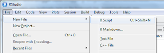
and you'll notice that an "Untitled1" file covers the auto dataset. Now we can start writing our do-file (okay, from now onwards I'll say R Script).
Task #3: Generate summary statistics
In the top left corner (not the console window) Type in summary(auto) and click run (near the top right hand corner of the editor. If you can't find it, press Ctrl+Enter and the code will run.
You'll observe some summary statistics in the Console screen. Some questions naturally arise.
Q: What if I only want one variable?
A: Try using the dollar sign. For example, summary(auto$price)
Q: But when I type "codebook" in Stata, it gives much more useful information such as number of missing values, etc. How can I generate these statistics?
A: Try the following commands:
install.packages('pastecs')
library(pastecs)
stat.desc(auto)
or if you prefer to look at a single variable (e.g. price), replace the last line with
stat.desc(auto$price)
Task #4: Generate correlation matrices
For preliminary data analysis, you may wish to generate correlation matrices. (These are done with corr or pwcorr in Stata).
For R, the analogous function is cor.
One may be tempted to type in cor(auto). However, RStudio displays the following error:
Error in cor(auto) : 'x' must be numeric
The non-numeric variables are preventing R from displaying the correlations. You can rectify this by issuing the following command instead:
cor(auto[sapply(auto, is.numeric)])
and the output should start like:
price mpg rep78 headroom trunk
price 1.0000000 -0.4685967 NA 0.1145056 0.3143316
mpg -0.4685967 1.0000000 NA -0.4138030 -0.5815850
rep78 NA NA 1 NA NA
headroom 0.1145056 -0.4138030 NA 1.0000000 0.6620111
What does sapply do? You would normally type "help sapply" in Stata, but the command is slightly different in R:
? sapply
The help file will load in the bottom right hand corner. Take a good look at it.
You may want to annotate your file at this point. For example, write a comment to remind yourself about what sapply does. In R, comments start with the pound sign ("#"). RStudio will display comments in green, just like Stata.
Task #5: List observations fulfilling certain criteria
You must be itching to find R's version of Stata's list function. It's just a different word:
To list the entire dataset:
print(auto)
To list only cars with gear ratio above 3.8:
print(subset(auto, subset = gear_ratio>3.8))
To list only foreign cars:
print(subset(auto, subset = foreign=="Foreign"))
To list only cars with gear ratio above 3.8 and mpg above 30:
print(subset(auto, subset = gear_ratio>3.8 & mpg > 30))
You've learned five crucial tasks. Part 2 will teach you five more key tasks!
Stata's advantage is that it has a wide variety of pre-programmed functions. These functions are not only easy to learn, but also easy to use. However, trying anything that is not pre-programmed (e.g. creating your own algorithm) is going to be difficult. This is much less difficult in R.
How, then, can a veteran Stata user convert to R? Here's a useful guide to mastering the basics.
If you haven't already, download the R program from the R website. Next, install RStudio.
What is RStudio?
You may have heard that the R interface is very plain, with pretty much only a command line to enter your commands (see below):

In contrast, the RStudio interface is much more intuitive:

Source: rprogramming.net
Looks just as good as Stata - in fact, probably better. So after you've finished downloading and installing it, your screen should be something like this:


Task #1: Import and open a Stata dataset
Let's take Stata's famous auto dataset, which you may have heard of. (To access this in Stata, simply type "sysuse auto.dta")
Let's take Stata's famous auto dataset, which you may have heard of. (To access this in Stata, simply type "sysuse auto.dta")
Method #1:
Open up Stata and load the auto dataset. Then save the auto dataset as a CSV file. Preferably name it auto.csv. If you don't have access to Stata now, here's a link to a CSV file.
Then go to RStudio and click Tools > Import Dataset > From Text File...
Below is a screenshot if you're not sure what to click.

You'll then encounter this dialog box.

Make any necessary changes (e.g. change "Heading" to Yes). Then click on "Import" on the bottom right hand corner. Your screen should look like this:

Look at the bottom left corner of the above screen. Notice how RStudio automatically generates the required command (just like Stata)? Also, RStudio automatically presents the data in the top left hand corner of the screen.
Method #2:
Install the package 'foreign', and then use this package to directly import a dta file
I'll leave this as an exercise, but will give some hints. You should start off with the following commands:
install.packages('foreign')
package(foreign)
Google if you're unsure how to continue!
(Another technical note: Since I am using RStudio here, I let blue Courier text denote commands and red text denote R's output. This is the opposite of other blog posts.)
Task #2: Create an R Script (aka 'do-file')
Recall how Stata had do-files? In R, you have R scripts. Just like do-files, these are simply text files containing commands.
Click File > New File > R Script

Task #3: Generate summary statistics
In the top left corner (not the console window) Type in summary(auto) and click run (near the top right hand corner of the editor. If you can't find it, press Ctrl+Enter and the code will run.
You'll observe some summary statistics in the Console screen. Some questions naturally arise.
Q: What if I only want one variable?
A: Try using the dollar sign. For example, summary(auto$price)
Q: But when I type "codebook" in Stata, it gives much more useful information such as number of missing values, etc. How can I generate these statistics?
A: Try the following commands:
install.packages('pastecs')
library(pastecs)
stat.desc(auto)
or if you prefer to look at a single variable (e.g. price), replace the last line with
stat.desc(auto$price)
Task #4: Generate correlation matrices
For preliminary data analysis, you may wish to generate correlation matrices. (These are done with corr or pwcorr in Stata).
For R, the analogous function is cor.
One may be tempted to type in cor(auto). However, RStudio displays the following error:
Error in cor(auto) : 'x' must be numeric
The non-numeric variables are preventing R from displaying the correlations. You can rectify this by issuing the following command instead:
cor(auto[sapply(auto, is.numeric)])
and the output should start like:
price mpg rep78 headroom trunk
price 1.0000000 -0.4685967 NA 0.1145056 0.3143316
mpg -0.4685967 1.0000000 NA -0.4138030 -0.5815850
rep78 NA NA 1 NA NA
headroom 0.1145056 -0.4138030 NA 1.0000000 0.6620111
What does sapply do? You would normally type "help sapply" in Stata, but the command is slightly different in R:
? sapply
The help file will load in the bottom right hand corner. Take a good look at it.
You may want to annotate your file at this point. For example, write a comment to remind yourself about what sapply does. In R, comments start with the pound sign ("#"). RStudio will display comments in green, just like Stata.
Task #5: List observations fulfilling certain criteria
You must be itching to find R's version of Stata's list function. It's just a different word:
To list the entire dataset:
print(auto)
To list only cars with gear ratio above 3.8:
print(subset(auto, subset = gear_ratio>3.8))
To list only foreign cars:
print(subset(auto, subset = foreign=="Foreign"))
To list only cars with gear ratio above 3.8 and mpg above 30:
print(subset(auto, subset = gear_ratio>3.8 & mpg > 30))
You've learned five crucial tasks. Part 2 will teach you five more key tasks!
Saturday, June 13, 2015
Introduction to R for Excel users
You've been using Excel a lot, but are new to R. You're wondering how to transition from Excel to R smoothly. If so, this post is for you.
First, open the R interface and you should reach this screen:

manufacturer model displ year cyl trans drv cty hwy fl class
1 audi a4 1.8 1999 4 auto(l5) f 18 29 p compact
2 audi a4 1.8 1999 4 manual(m5) f 21 29 p compact
3 audi a4 2.0 2008 4 manual(m6) f 20 31 p compact
...
232 volkswagen passat 2.8 1999 6 auto(l5) f 16 26 p midsize
233 volkswagen passat 2.8 1999 6 manual(m5) f 18 26 p midsize
234 volkswagen passat 3.6 2008 6 auto(s6) f 17 26 p midsize
As you can see, there are 234 observations of popular cars from 1999 to 2008.
How can we tell R to sort the data accordingly? We can use the order command:
R processes the command and outputs:
manufacturer model displ year cyl trans drv cty hwy fl class
1 audi a4 1.8 1999 4 auto(l5) f 18 29 p compact
2 audi a4 1.8 1999 4 manual(m5) f 21 29 p compact
5 audi a4 2.8 1999 6 auto(l5) f 16 26 p compact
...
Whoops! Notice that the default is to output in an ascending order. To fix this, simply add a minus sign in front of mpg$year:
Challenge 1: Sort by year, and then displ
Challenge 2: Sort by year, and then manufacturer (this is a little harder because manufacturer is a string variable)
auto(av) auto(l3) auto(l4) ...
5 2 83 ...
auto(s6) manual(m5) manual(m6)
16 58 19
How can we shave off the items in brackets?
There are several methods available. Some methods are short and sweet but rely on a crucial aspect of the dataset we're working on now (e.g. there are only auto and manual cars). Others are longer, but are more generalizable (i.e. the methods can be applied to other datasets as well).
First, open the R interface and you should reach this screen:

We're going to use a package called ggplot2. (Think of it as an "add-on" to R). In R, you need to load packages through the library function, so type in the following command:
library(ggplot2)This package contains the dataset mpg that we need to use:
mpgYou should see lots of lines of text after typing the above command. I've copied and pasted the start and end:
manufacturer model displ year cyl trans drv cty hwy fl class
1 audi a4 1.8 1999 4 auto(l5) f 18 29 p compact
2 audi a4 1.8 1999 4 manual(m5) f 21 29 p compact
3 audi a4 2.0 2008 4 manual(m6) f 20 31 p compact
...
232 volkswagen passat 2.8 1999 6 auto(l5) f 16 26 p midsize
233 volkswagen passat 2.8 1999 6 manual(m5) f 18 26 p midsize
234 volkswagen passat 3.6 2008 6 auto(s6) f 17 26 p midsize
As you can see, there are 234 observations of popular cars from 1999 to 2008.
Sorting
Obviously, the variable "year" contains information about the year of a specific model. Let's say we want to see the latest models first.How can we tell R to sort the data accordingly? We can use the order command:
mpg[order(mpg$year)]Notice that mpg is again a reference to the mpg dataset, and by using the square brackets ([]) I'm saying I want to access certain list members, or arrange them in a specific way. the function order is key here: it tells R to sort the data. Finally, mpg$year says, "Sort according to the year variable in the mpg dataset".
R processes the command and outputs:
manufacturer model displ year cyl trans drv cty hwy fl class
1 audi a4 1.8 1999 4 auto(l5) f 18 29 p compact
2 audi a4 1.8 1999 4 manual(m5) f 21 29 p compact
5 audi a4 2.8 1999 6 auto(l5) f 16 26 p compact
...
Whoops! Notice that the default is to output in an ascending order. To fix this, simply add a minus sign in front of mpg$year:
mpg[order(-mpg$year)]Now you should get what you want.
Challenge 1: Sort by year, and then displ
Challenge 2: Sort by year, and then manufacturer (this is a little harder because manufacturer is a string variable)
Manipulating variables
The variable cty refers to "miles per gallon for city driving". Likewise, hwy refers to "miles per gallon for highway driving". Let's say I'm sending this dataset to a European friend, and I'd like to convert them into liters per 100 km.
Working through the math, we realize that 1 mile per gallon is 235 liters per 100 km.
It's easy to do the conversion:
mpg$hwy <- mpg$hwy * 235
mpg$cty <- mpg$cty * 235
If we were driving on the highways 40% of the time, and driving within the city 60% of the time, it would be easy to construct a weighted average:
mpg$wtavglp100k <- mpg$hwy*0.4 + mpg$cty*0.6
lp100k is shorthand for liters per 100 km.
Rename variables
Recall we had done some metric conversion for our European friend. How can we remind ourselves that we've done these conversion?
The following commands should make clear what units the variables are in:
names(mpg)[8] <- "lp100k_cty"
names(mpg)[9] <- "lp100k_hwy"
Capturing part of a variable
Let's take a look at the trans variable closely:
summary(mpg$trans)outputs
auto(av) auto(l3) auto(l4) ...
5 2 83 ...
auto(s6) manual(m5) manual(m6)
16 58 19
How can we shave off the items in brackets?
There are several methods available. Some methods are short and sweet but rely on a crucial aspect of the dataset we're working on now (e.g. there are only auto and manual cars). Others are longer, but are more generalizable (i.e. the methods can be applied to other datasets as well).
Method 1
mpg$transmission <- substring(mpg$trans,1,4)
mpg$transmission[mpg$transmission=="manu"] <- "manual"
Method 2
use gsub, which substitutes an expression for another.
Note: we need to use double backslash (i.e. \\) because "(" is considered to be a metacharacter. (Think of a metacharacter as a special character).
mpg$trans <- gsub(\\(.*$","",mpg$trans) # best
or
mpg$trans <- gsub(\\(..\\)","",mpg$trans)
or
mpg$trans <- gsub(\\([a-z][a-z0-9]\\)","",mpg$trans)
In the first command, .*$ pick up everything after the opening bracket (. Likewise, ..\\) and ([a-z][a-z0-9]\\) do the same. This document produced by Svetlana Eden is an excellent guide to knowing the finer details of what was done.
mpg$trans <- substr(mpg$trans,0,a-1) # drops everything including and after (
rm(a) # removes the variable a, which was intended to be a temporary variable
Using any of these methods, all the text following ( is now deleted. We can verify this by typing mpg$trans or (better) if we want to be doubly sure, type unique(mpg$trans)
In the first command, .*$ pick up everything after the opening bracket (. Likewise, ..\\) and ([a-z][a-z0-9]\\) do the same. This document produced by Svetlana Eden is an excellent guide to knowing the finer details of what was done.
Method 3
a <- regexpr("\\(",mpg$trans) # finds the position of (mpg$trans <- substr(mpg$trans,0,a-1) # drops everything including and after (
rm(a) # removes the variable a, which was intended to be a temporary variable
Using any of these methods, all the text following ( is now deleted. We can verify this by typing mpg$trans or (better) if we want to be doubly sure, type unique(mpg$trans)
Subscribe to:
Posts (Atom)