Google Maps for the uninitiated

Are you a regular user of Google Maps, but are wondering how to use it in R? If so, this post is for you.

You'll need to install several libraries and load them:

install.packages(raster)
install.packages(sp)
install.packages(dismo)
install.packages(XML)

library(raster)
library(sp)
library(dismo)
library(XML)

As a reminder, packages are "add-ons": collections of functions, data, etc. which can be used in R.

But plotting is surprisingly simple All you need is an internet connection:

plot(gmap('malaysia'))

gmap calls the Google Maps function, and then I specify what map I want (in this case, Malaysia). Don't forget the quotes, although it doesn't matter whether you use double quotes or single quotes. R then loads Google Map's view of Malaysia.

Notice that Malaysia is divided into two halves. (Observe there are two labels of Malaysia, one on the left side of the diagram, and the other, on the right.)

Most Malaysians, however, stay in the western half of Malaysia. The capital Kuala Lumpur is in the western half of Malaysia too. Thus I might only want to see the western half.

In this case, I can click

myRegion <- drawExtent() 

Then, click twice to draw a rectangle around the western half:

For example, you can click at the bottom left hand corner, and the top right hand corner (which is what I did). Or you can click at the bottom right hand corner, and the top left hand corner. (Notice, you only need to specify two opposite ends of a rectangle to define a rectangle).

R then records myRegion as the red box. To get better view, type

plot(gmap(myRegion)) # without quotes, since it is a variable.

Recall once again that everything after the pound (#) sign is a comment and will not be processed by R.
And there you have it: a better view of west Malaysia.

Now, let's see how we can plot data onto Google Maps.

Download this file and place it in your working directory. (If you're unsure of you're working directory, type getwd()and see what comes up)

The file is a CSV file containing crime data in Charlotte, North Carolina, USA.

Let's load it into memory and plot the points:

mydata<-read.table("CLTCrime.csv",sep=",", header=TRUE)  #this loads the CSV file. make sure the CSV file is in your working directory.

names(mydata) # gives you the variable names

coordinates(mydata) <- c("longitude","latitude") # sets the spatial coordinates of each observation (as the longitude and latitude)

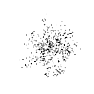
plot(mydata) # scatterplot of crime points without map

We've plotted the geographic location of each crime incident in Charlotte. Much of the crime occurs in a central location - probably Charlotte's downtown. However a big piece of the picture is missing: a map of Charlotte.

Let's add on a map of Charlotte:

crs.geo <- CRS("+proj=longlat +ellps=WGS84 +datum=WGS84")  # describes the projection system you want to use.

proj4string(mydata) <- crs.geo # sets projection attributes

gbmap <- gmap(mydata) # gives the map which contains all the data points. (happens to be charlotte)

mydata.merc<-Mercator(mydata) # Sets the data to mercator. This is necessary because Google Maps are in Mercator projection.

plot(gbmap) # produces the map of Charlotte

points(mydata.merc,pch=20,col="steelblue") # superimposes points.

legend("bottomleft",inset=.07,bg="white", legend="CrimeEvents",pch = 20, col="steelblue") #adds a legend 

The commands might be confusing to most, even after I've annotated comments. The first three commands are mainly technical. Together, they create the map which will be sufficient to contain the points in the dataset "mydata". Notice that if "mydata" had contained crime in the US, the map generated would have been that of the US.

The command mydata.merc<-Mercator(mydata)adjusts the coordinates to fit the Mercator convention, since that's what Google Maps uses. Subsequently plot(gbmap) and

points(mydata.merc,pch=20,col="steelblue") add the map and superimpose points respectively. Finally, a legend is added.  

Look at the beautiful map that R and Google Maps produced!

There is another (perhaps more elegant) way of doing this:

library(googleVis) # if you don't have this package, then run install.packages('googleVis') first
mydata<-read.table("CLTCrime.csv",sep=",", header=TRUE)# change the directory as necessary
M1 <- gvisMap(mydata,"LatLong","Descrip")
plot(M1) # plots the map by loading it into a browser

gVisMap calls the Google Visualization API. The first argument, mydata, tells Google which dataset needs to be used. The second argument, LatLong, tells Google, "The location of each observation is contained within the LatLong variable in mydata.". The third argument, Descrip, tells Google, "For each observation, the value of the variable Descrip describes the observation". In other words, Descrip provides a description (or acts as a "label") of the crime that happened.

The command plot(M1) then opens a web browser and displays the following map:

If you actually did this exercise, you would be able to click on each crime report to discover what crime was reported (that's the value of the variable "Descrip")

Congratulations on your first use of Google Maps in R!